|
|
|
In order to digitally recreate real-world scenes for video games, movies, AR/MR/VR and industrial simulations, creators need visually convincing representations of fluids. Scientifically accurate simulations governed by complex equations are true to reality, but difficult to implement and are computationally expensive to use. In the following project, we explore the implications of speed, interpretability, and interactivity of fluid simulations for viewers and programmers. Our mathematical implementation is based on Muller et al.’s Position based dynamics (2007) and the follow-up paper Macklin and Muller’s Position Based Fluids (2013), which involves understanding the physics of individual particles and calculating particle positions from density and other parameters. We modified Project 4 rendering GUI to support particles instead of cloth grids and extended functionality to allow for three-dimensional grid parameters for more complexity in simulation. To execute fast nearest neighbor search, we utilized the nanoflann library during our intermediate calculations. Although we were not able to implement a water shader and the machine learning speed-up that we hoped for, we believe our results in creating a real-time renderer that only uses CPU computation aligns to our original goals for speed and interpretability.
Before implementing the specifics for fluid simulation mathematics, we prepared for integration to our current system via an object-oriented approach and interacted with pre-made files from Project 4. We changed functionalities to provide flexibility toward creating different .json set-up files and to create applicable visualization of individual particles.
Our two main goals here was to provide increased alignment to variables introduced within Position Based Fluids (2013) and new methods of handling particle rendering by the Project 4 GUI. To respond to the first point, we added in Vector3D dp, Particle *particle, double lambda, Vector3D velocity_star, and Vector3D position_star to follow the same attribute requirements from the paper. For the second motive, we created a Particle class to allow for quick renders between simulation steps by avoiding re-instantiation of sphere meshes that represent each particle. This was then associated with our PointMass objects through the buildGrid method, as we assigned each new particle to each PointMass.
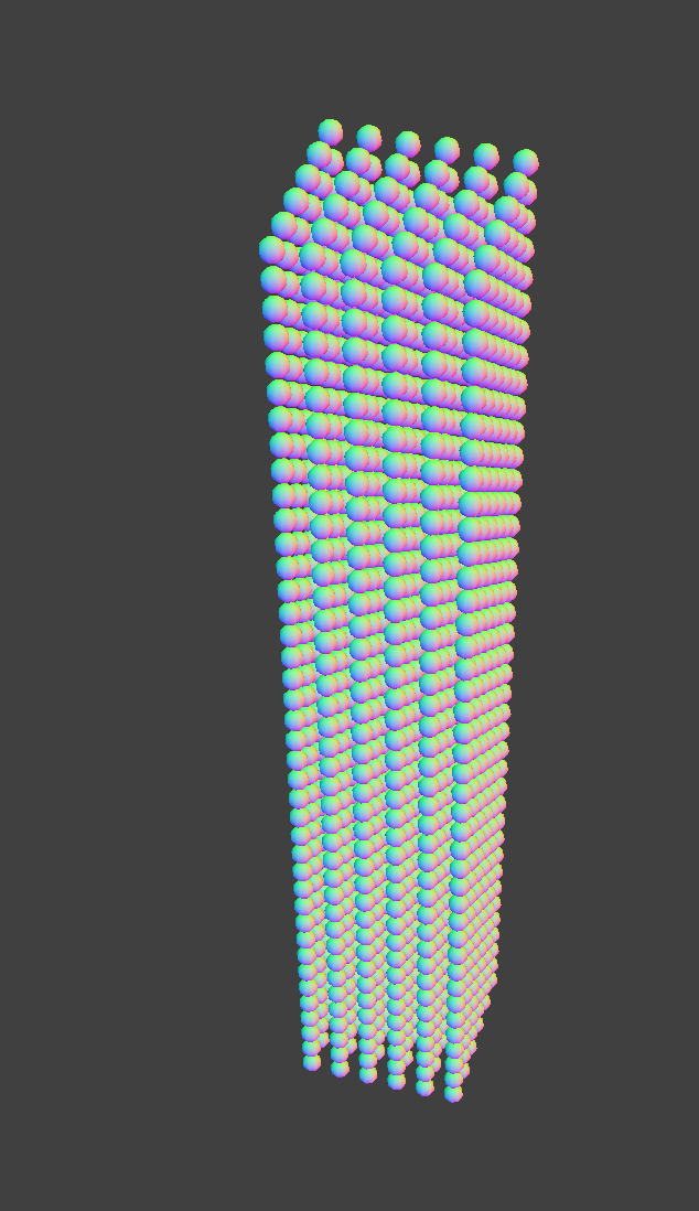
3D VOLUME GRIDS: Furthermore, we allowed for a 3D volume of particles to be created, as opposed to a 2D grid done in Project 4 to more accurately simulate fluids, since fluids are not realistically represented by thin sheets.This was accomplished through adding a third attribute num_depth_points and an extra loop over the buildGrid method. To center our 3D particle volume, we offset the spacing by subtracting half the number of points along that dimension. Dynamically calculating the spacing through dividing the dimension attributes by the number of points, we kept constant spacing across each respective dimension.

|
|
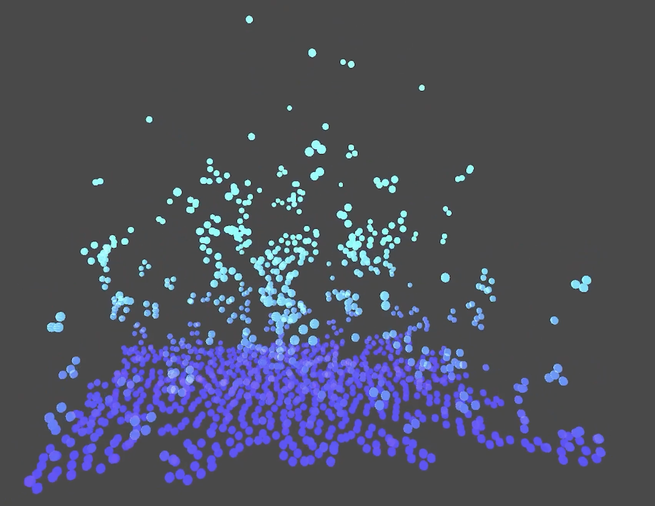
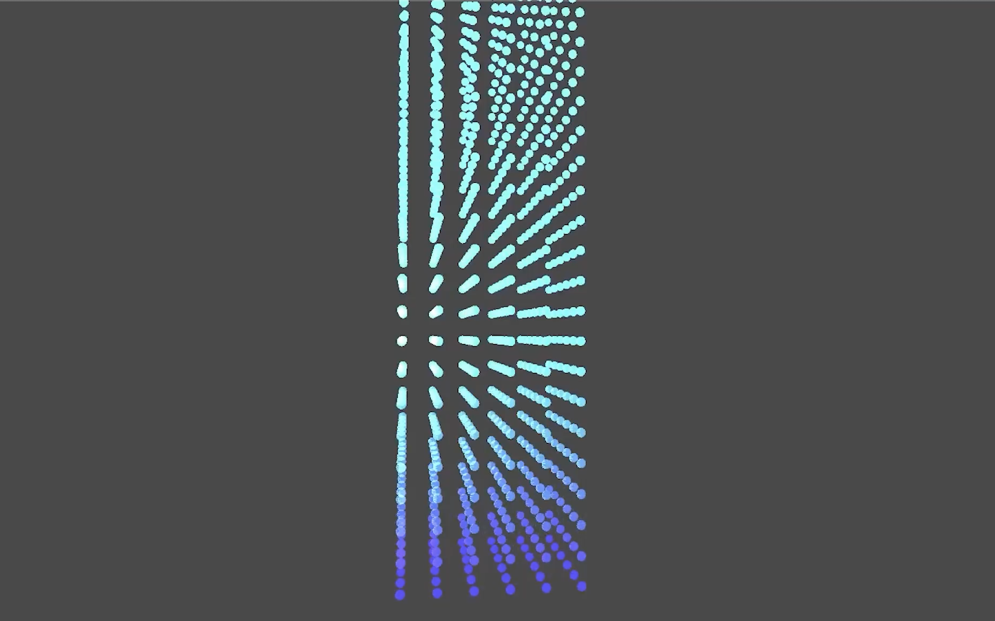
COLOR-CODED SPHERE RENDERINGS: To allow for visual communication of particle position, we varied the color depending on the Y positions of each particle. We modified the Default.vert, Phong.frag, and Wireframe.frag files to include color attributes and changed the sphere_drawing.cpp file to provide the colors to our spheres.
|
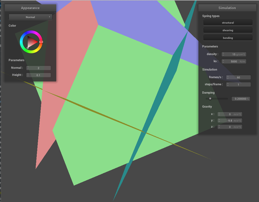
CREATING NEW SCENES: We wanted to be able to create different surfaces for our particles to interact with. We modified the way that .JSON files were parsed to have more control over what scenes we created. The two scenes we ended up making was 1. a 4-walled room and 2. a slanted alley to provide fluid particle collisions with containers.
|
The algorithm described by Macklin and Muller relies heavily on identifying the neighboring particles near a given particle to compute its next position. Naive search throughout all points is inefficient and antagonistic to our goal of achieving fast rendering, so we looked into clustering methods to improve performance. At first, we experimented with spatial hashing that we completed in Project 4, but found it to be extremely buggy, as grid lines and regularities in particle movement resulted. Via the suggestion of TA Utkarsh, we utilized nanoflann, which finds nearest neighbors using a KDTree approach with point clouds utilizing a search radius.
In Cloth.cpp, we begin building our point cloud to search for nearest neighbors, creating a vector of PointMasses pmNeighbors to hold the list of neighbors that correspond to a PointMass object in row-major order. We utilize nanoflann’s radius search function to extract neighbors and prepare for usage in the following algorithm components.
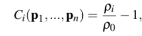
Position Based Fluids provides an approach that does not require direct force manipulations, and utilizes position changes to implicitly convey the forces at play. This is helpful with overall stability and density issues from previous work with Smoothed Particle Hydrodynamics (SPH), Monaghan (1992, 1994). The following set of equations make sure density is constant across the movement of the particle fluid system.
|
|
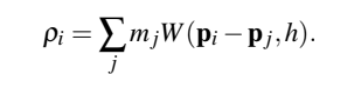
After finding the associated neighbors of each particle during each timestep, we proceed to implementing the equations above, which describes the density of a particle and its corresponding density constraint C_i . This step involves the Poly6 kernel, W, which is as follows:
Function W(Vector3D r, double h)
if 0 < norm(r) < h:
     Return 315.0 / (64.0 * PI * pow( h, 9.0)) * pow(h * h - norm(r)  * norm(r) , 3);
Return 0;
|
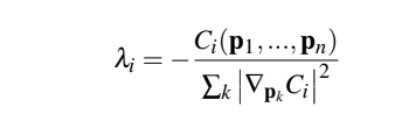
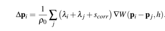
Next we account for neighborhood density corrections, lambda. This is different from the individual particle density constraints in that it provides context to other particle interactions. We utilize the Spiky kernel gradW to evaluate the denominator and added an epsilon, 1e-5, term in the denominator to prevent instability. The Spiky kernel is as follows:
Function gradW(Vector3D r, double h)
if 0 < norm(r) < h:
      Return -45.0f / (PI * pow(h, 6)) * pow(h - norm(r), 2) / (norm(r) + 1e-5) * r;
Return 0;
|
|
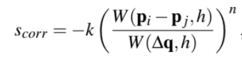
Finally, we used this quantity to account for the total position update of a given particle, after adding in a corrective term to prevent issues associated with clustering of particles.
|
c = 0.001.
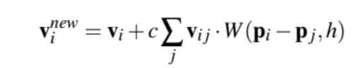
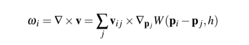
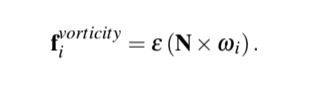
To account for turbulent motion and energy conservation properties of simulation, we implemented vorticity confinement for replacing lost energy.
|
|
We calculated the vorticity element at a given particle’s location and then applied a corrective force to the forces of our current particle and updated its respective velocity
Each of these quantities were then integrated into our overall simulation step. We utilized a set amount of simulation steps and in each loop, we do the following:
Accumulate lambda values through iterating through point masses and their neighbors
Calculate delta p_i, the change in position for each particle through their relationship to their neighbors
Update position_star with delta p_i
Check for collisions with external object
Update velocity based on current position_star and existing position
Account for viscosity and vorticity confinement for velocity updates
Update positions
Below are our results. The first video displays a stream of fluid flowing into a box-like container. The second displays the motion into a narrow alley. Our renders could be accomplished in real time, with 1440 points rendered with various colors at 60 frames per second.
Macklin, Miles and Matthias Muller. Position Based Fluids (2013). NVIDIA.
Muller, Matthias, David Charypar, and Markus Gross. Particle-Based Fluid Simulation for Interactive Applications (2003). Department of Computer Science, Federal Institute of Technology Zurich (ETHZ), Switzerland.
Muller, Matthias, Bruno Heidelberger, Marcus Hennix, John Ratcliff. Position Based Dynamics (2007). ScienceDirect.
Schechter, Hagit and Robert Bridson. Ghost SPH for Animating Water (2012). ACM Trans. Graph.
Adnaan worked on lots of the core functionality in the codebase. He helped implement the 3D initialization of fluid particles and box scenes. He also worked with Lily to implement the incompressiblity constraint and all of its equations, and he implemented tensile instability. Adnaan also worked with shaders to develop the height-based coloring of particles in the final renders.
Lily worked with Adnaan via the CLion coding Liveshare platform to implement the initial functionality of the paper, putting together the skeleton needed for calculating density, confinement coefficients, and neighboring particle interactions. She also contributed to modifying the box scene and prototyping the 3D support in the buildGrid function. Lily was responsible for creating the majority of the slides for the milestone and final deliverables, and wrote the final writeup.
Mark worked with Sophia to implement and debug viscosity and vorticity confinement over Visual Studio live share. Mark modified the json scene interpreting code to support scenes with multiple collidable planes. He also helped write the project proposal and the milestone report. In collaboration with Lily, Mark created two box scenes to contain the simulated fluid.
Sophia worked with Mark to implement viscosity and vorticity confinement over Visual Studio live share.